Hyperbolic Equation Solution by a Second Order Upwind Approximation by MATLAB

Let's assume that the temperature distribution inside a pipe is governed by the following one dimensional unsteady hyperbolic partial-differential-equation

Tt + u Tx = 0

Consider negligible heat diffusion and the initial velocity u is, 0.1 cm/s. The boundary conditions are described below:

T(x, 0) = 200 x;       0 ≤ x ≤ 0.5

T(x, 0) = 200 (1 – x);       0.5 ≤ x ≤ 1

Develop an algorithm in MATLAB to solve this problem using the second-order approximation in time and the second-order upwind approximation in space. Consider, Δx = 0.05 cm; Δt = 0.05. 

The following MATLAB program develops the second order upwind method to solve the given one-dimensional unsteady hyperbolic convection equation.


% Hyperbolic equation - Convection equation: Upwind Method
close all;
clc;

% Input Properties from Problem
L=1.0; % (dimension in cm)
Lmax=5.0;
alpha=0.01;
u=0.1; % (dimension in cm/s)
Tt=10; % Simulation Time Period

% Mesh/Grid size
dx=0.05;
dt=0.05;

c=u*dt/dx; % Depends on dt values
d=alpha*((dt/dx)^2.0);

% Matrix Parameters

imax=(Lmax/dx)+1; % Array dimension along the width
tmax=(Tt/dt); % Array dimension along the height
ndim=imax-2;
tdim=tmax-2;

% Total no of iterations
iteration=10000;

% Convergence Criterion
tolerance=0.000001;

% Array and Variables
% a = Matrix of Coefficients A(i,j)
% b = Right Side Vector, b(i)
% x = Solution Vector, x(i)

% Initial Condition
f(:,1)=0.0;
for i=1:imax-2
    x(i)=(i-1)*dx;
   
    if x(i)<=1.0
        f(i,1)=0.0;
    end
    if x(i)>1.0 && x(i)<=1.5
        f(i,1)=200*(x(i)-1.0);
    end
    if x(i)>1.5 && x(i)<=2.0
        f(i,1)=200*(L-x(i)+1.0);
    end
    if x(i)>2.0
        f(i,1)=0;
    end
end

fprintf('imax = %f\n',imax);
fprintf('c=%f\n',c);

% Upwind Method

for t=1:tmax
    time(t+1)=(t)*dt;
    for i=2:imax-2
        % Second Order Approximation
       f(i,t+1)=f(i,t)-c*(f(i,t)-f(i-1,t))-0.5*c*(1.0-c)*(f(i,t)-2.0*f(i-1,t)+f(i-2,t));
    end
end

hold on
plot(x,f(:,1))
plot(x,f(:,find(time==1)),'o-')
plot(x,f(:,find(time==5)),'o-')
plot(x,f(:,find(time==10)),'o-')

xlabel('x, cm')
ylabel('Temperature, C')
legend('t=0s','t=1s','t=5s','t=10s')
title ('c=0.1')

Program Output:

Second-order approximation in time and second-order upwind approximation in space:
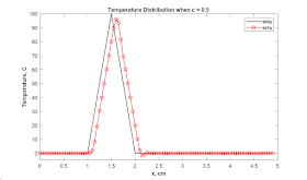
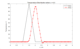
Temperature Distribution in Pipe for Different t and c Values

Temperature Distribution in Pipe for Different t and c Values

Temperature Distribution in Pipe for Different t and c Values

Temperature Distribution in Pipe for Different t and c Values

Temperature Distribution in Pipe for Different t and c Values

Temperature Distribution in Pipe for Different t and c Values

Hyperbolic Equation Solution by a First Order Upwind Approximation by MATLAB

Let's assume that the temperature distribution inside a pipe is governed by the following one dimensional unsteady hyperbolic partial-differential-equation:

Tt + u Tx = 0

Consider negligible heat diffusion and the initial velocity u is, 0.1 cm/s. The boundary conditions are described below:

T(x, 0) = 200 x;       0 ≤ x ≤ 0.5

T(x, 0) = 200 (1 – x);       0.5 ≤ x ≤ 1

Develop an algorithm in MATLAB to solve this problem using the first-order approximation in time and the first-order upwind approximation in space. Consider, Δx = 0.05 cm; Δt = 0.05. 

The following MATLAB program develops the first-order upwind method to solve the given one-dimensional unsteady hyperbolic convection equation.


% Hyperbolic equation - Convection equation: Upwind Method
close all;
clc;

% Input Properties from Problem
L=1.0; % (dimension in cm)
Lmax=5.0;
alpha=0.01;
u=0.1; % (dimension in cm/s)
Tt=10; % Simulation Time Period

% Mesh/Grid size
dx=0.05;
dt=0.05;

c=u*dt/dx; % Depends on dt values
d=alpha*((dt/dx)^2.0);

% Matrix Parameters

imax=(Lmax/dx)+1; % Array dimension along the width
tmax=(Tt/dt); % Array dimension along the height
ndim=imax-2;
tdim=tmax-2;

% Total no of iterations
iteration=10000;

% Convergence Criterion
tolerance=0.000001;

% Array and Variables
% a = Matrix of Coefficients A(i,j)
% b = Right Side Vector, b(i)
% x = Solution Vector, x(i)

% Initial Condition
f(:,1)=0.0;
for i=1:imax-2
    x(i)=(i-1)*dx;
   
    if x(i)<=1.0
        f(i,1)=0.0;
    end
    if x(i)>1.0 && x(i)<=1.5
        f(i,1)=200*(x(i)-1.0);
    end
    if x(i)>1.5 && x(i)<=2.0
        f(i,1)=200*(L-x(i)+1.0);
    end
    if x(i)>2.0
        f(i,1)=0;
    end
end

fprintf('imax = %f\n',imax);
fprintf('c=%f\n',c);

% Upwind Method

for t=1:tmax
    time(t+1)=(t)*dt;
    for i=2:imax-2
        % First Order Approximation
        f(i,t+1)=f(i,t)-c*(f(i,t)-f(i-1,t));
    end
end

hold on
plot(x,f(:,1))
plot(x,f(:,find(time==1)),'o-')
plot(x,f(:,find(time==5)),'o-')
plot(x,f(:,find(time==10)),'o-')

xlabel('x, cm')
ylabel('Temperature, C')
legend('t=0s','t=1s','t=5s','t=10s')
title ('c=0.1')


Program Output:


Temperature Distribution inside Pipe for Various c and t

Temperature Distribution inside Pipe for Various c and t

Temperature Distribution inside Pipe for Various c and t

Temperature Distribution inside Pipe for Various c and t

Temperature Distribution inside Pipe for Various c and t

Temperature Distribution inside Pipe for Various c and t

Adams-Bashforth Method with RK2 as a Start-up Scheme in MATLAB

Let's consider the following differential equation:

y'' + 10 y' + 500y = 0

Where, the initial conditions are,

y(0) = -0.025, and y'(0) = -1


We will solve this differential equation using a multi-step methodAdams-Bashforth, where second order Runge-Kutta approach (RK2) is added as a start-up scheme in the algorithm. 

MATLAB Program:
The following MATLAB program implements the Adams-Bashforth method with initialization with RK2 method.

close all;

clc;
h = 0.02;     % Step size
Tmax = 0.5;    % Maximum time
N = Tmax / h;  % Maximum number of steps
alpha=0.5;
t = linspace(0,0.5,N+1);  % Time range

% Analytical solution of the differential equation
y_real = -(((9.*sqrt(19))/760).*exp(-5.*t).*sin(5.*sqrt(19).*t)) - ((1/40).*exp(-5.*t).*cos(5.*sqrt(19).*t));
plot(t,y_real);
hold on

%Numerical solution
f=@(t,y) [y(2); -500*y(1)-10*y(2)]; % Governing system of equations

% Initial Conditions
Y = [-0.025; -1];
% Initialization with second order Runge-Kutta method
k1 = h.*f(t(1),Y(:,1));
    k2 = h.*f(t(1)+alpha.*h, Y(:,1)+alpha.*k1);
    Y(:,2) = Y(:,1) + (1-1/2/alpha).*k1 + k2/2/alpha;

% Second Order Adams-Bashforth method steps
for i=2:N
    Y(:,i+1) = Y(:,i) + 3/2*h*f(t(i),Y(:,i)) - h/2*f(t(i-1),Y(:,i-1));
end

plot(t,Y(1,:),'o:')
legend('Exact Solution','Adams-Bashforth Solution','Location','NorthEast')
title('When h = 0.02')
xlabel('t')
ylabel('y')


Program Output:
The following plot shows the numerical and analytical solution of the differential equation with two different step sizes with respect to time.

Showing results for Adams-Bashforth method when step is 0.02

Showing results for Adams-Bashforth method when step is 0.01