Some Frequently used Interpolation Tools by MATLAB

Interpolation is a very essential tool in any areas of research these days. Whether you are analyzing your data or deriving equations to represent a system, interpolation plays an immense role in these works. Luckly, MATLAB has some built-in commands for basic data fitting. Not only that, you may also create your own function and use it stand alone or in combination of calling some MATLAB commands. In this article, I am going to discuss three basic techniques for basic data fitting. They are,

• Polynomial Interpolation
• Piecewise Linear Interpolation
• Cubic Spline Interpolation

Polynomial Interpolation: Polynomial interpolation is one of the most basic interpolation tools. The first step would be to learn this technique manually as it would provide us insights into the fundamentals prior to using MATLAB built-in features. The idea is that a polynomial of n degree would pass through all the (n+1) points if we apply the technique of polynomial interpolation. Let us begin with an example to strengthen the concept. 

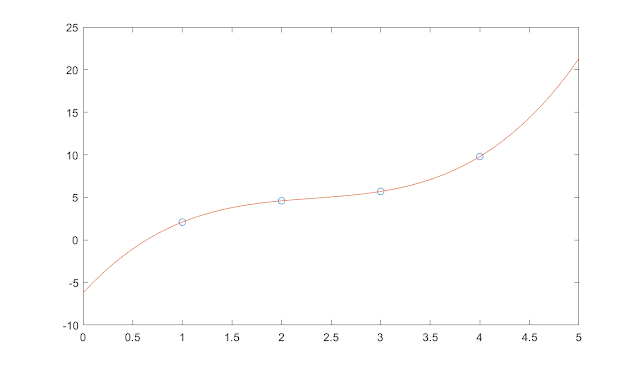
Let’s say, we have data points: (1, 2.1), (2, 4.6), (3, 5.7) and (4, 9.8). The goal is to fit a polynomial that would pass through all these points. We may consider these points as (x₁, y₁), (x2, y2), (x3, y3), and (x4, y4) where x refers to the horizontal axis and y refers to the vertical axis.

Data points from the example

Now, let's define a general polynomial equation. The following is the n-th order polynomial:



If we extend the general polynomial, it looks like the following as,

And, in matrix form, we may arrange these equations nicely as follows,

For our example problem, we have 4 data points, which means that we will have four equations. The right side vector b is for the vertical (y-axis) data points. The left side nxn matrix is for the horizontal (x-axis) data points. But, there is a question. The horizontal data points are not in a squared matrix, specifically, it is now in 1x4 form; so, how could we represent the data as in a 4x4 matrix for our example? The following figure shows the current configuration:

We can write a simple MATLAB program to make that 4x4 matrix. The following codes will generate a square matrix from a single row matrix.

% Generation of a Polynomial Matrix

x=[1 2 3 4]; % Sample x data points

n = length(x); 

A = zeros(n,n);

 

for i=1:n

% Creating polynomial matrix

for j=1:n

% nth degree polynomial passing through (n-1) points

A(i,j) = x(i).^(j-1);

end

end

disp(A)

After implementing the above program, we will have the following refined equations, which we can solve by Gaussian elimination to find the value of the unknown coefficients, a.

Now, using the Gaussian elimination, the unknown parameters are,

So, the polynomial equation that will pass through all the four points is,

If we plot, the above equation fits and passes through all the points. 

So far, the mathematics behind polynomial interpolation has been discussed. Good news! MATLAB has a built-in polynomial interpolation feature. We can use the feature easily. You can access the built-in function from the command prompt shown as below,

>> x = [1; 2; 3; 4];

>> y =[2.1; 4.6; 5.7; 9.8];

>> polyfit(x,y,3)

ans =

-6.2

12.667

-5.10

0.7333

'polyfit' is the built-in command in MATLAB that uses the same technique shown earlier. 

Piecewise Linear Interpolation: When we have more data points to fit, polynomial interpolation does generate too much oscillations in curve fitting. In this case, we may use the MATLAB built-in command 'interp1' for one dimensional piecewise linear interpolation. For our four data points example, we may write few lines in MATLAB command prompt to access this feature.

>> x1 = [1;2;3;4];

>> y1 =[2.1; 4.6; 5.7; 9.8];

>> xx = 0:0.1:5;

yy = interp1(x1,y1,xx);

plot(x1,y1,'o',xx,yy)

Cubic Spline Interpolation: An improvement to one dimensional piecewise linear interpolation is the cubic spline interpolation. We may use the MATLAB built-in command 'spline' for it. For our four data points example, we may write few lines in MATLAB command prompt to access this feature.

>> x1 = [1;2;3;4];

>> y1 =[2.1; 4.6; 5.7; 9.8];

>> xx = 0:0.1:5;

yy = spline(x1,y1,xx);

plot(x1,y1,'o',xx,yy)

#Interpolation #PiecewiseLinear #CubicSpline #Matlab #Polynomial #Blog #Blogger

Vectorization in MATLAB: Use of Colon (:)

We are familiar with 'for loop' application in MATLAB. We may use many 'loops' to handle complex calculations. But, sometimes too many 'loops' cost computational time, which eventually affects the overall efficiency of the codings. In MATLAB, instead of looping, we may use the method of vectorization to skip some 'loops'. We may use the operator colon (:) in MATLAB to form vectors that alternately eliminates the 'loops'. Let's explain the method with a very simple example. For example, we would like to divide a square matrix (for our example, 5x5) with a scalar number. Below, there are three scenarios. At first, we can use 2 'for loops' to do the operation. Secondly, we can skip one 'for loop' by using a colon (:) for the columns of the matrix a. Finally, we can avoid all 'for loops', and use colons (:) for both rows and columns of the example matrix a.

2 'for loop':

i=1;

j=1;

n=5;

a=[1 2 3 4 5; 6 7 8 9 10; 1 2 3 4 5; 6 7 8 9 10; 1 2 3 4 5;];

 for i=1:n

     for j=1:n

     a(i,j) = a(i,j)./n;

     end

 end

 disp(a)

1 'for loop':

i=1;

j=1;

n=5;

a=[1 2 3 4 5; 6 7 8 9 10; 1 2 3 4 5; 6 7 8 9 10; 1 2 3 4 5;];

 for i=1:n

     

     a(i,j:n) = a(i,j:n)./n;

    

 end

 disp(a)

0 'for loop':

i=1;

j=1;

n=5;

a=[1 2 3 4 5; 6 7 8 9 10; 1 2 3 4 5; 6 7 8 9 10; 1 2 3 4 5;];

 

a(i:n,j:n) = a(i:n,j:n)./n;

disp(a)

In all the above cases, the results are the same. You may run the codes and check for yourself. The operation is pretty straightforward here. When colon (:) is first used between j and n,  we eliminate a 'for loop'. This colon (:) is considering all the elements in columns of the matrix a, which is equivalent to the 'loop' operation. The second colon (:), between i and n (i:n), takes all the row elements of the matrix a, and the operation is also same compared to using a 'for loop'. Below is the result for all three demonstrated cases.

    0.2000    0.4000    0.6000    0.8000    1.0000

    1.2000    1.4000    1.6000    1.8000    2.0000

    0.2000    0.4000    0.6000    0.8000    1.0000

    1.2000    1.4000    1.6000    1.8000    2.0000

    0.2000    0.4000    0.6000    0.8000    1.0000

This is a very simple example, and for this, you won't even realize the actual computational efficiency. But, imagine! you have very large matrices where numerous complex operations involved. In that case, you would be able to see the differences. 

#Vectorization #Matrix #ForLoop #UseofColon #Matlab #Blog #Blogger

Comparison between 4 and 8 Node Integration Elements in Finite Element Analysis

Let us assume a cantilever beam with one end fixed and the other end has 1 unit load acting vertically downward. The length and height of the beam are 5 and 1 unit respectively. The Young's modulus is 10,000 unit. At first, we will solve this problem analytically using the famous Euler-Bernoulli beam equation to find the deflection at the end of the beam. Next, we will use Abaqus with 4 node quadrilateral  reduced integration element. Then, we will solve the same problem using 8 node quadrilateral reduced integration element. Our goal is to see which element performs better in terms of convergence and accuracy for the finite element analysis (FEA) compared to the analytical solution.

The following Mathematica program solves the Euler-Bernoulli equation for the deflection at the tip.

(*Exact Solution of Euler-Bernoulli Cantilever Beam*)

Clear[y, P, x, X2, EI, L];

y[x];

(*Given Property Values*)

L = 5;

h = 1;

P = 1;

Ie = 1/12;

Ee = 10000;

EI = Ee*Ie;

theta = D[y[x], x];

V = EI*D[y[x], {x, 3}];

M = EI*D[y[x], {x, 2}];

y1 = y[x] /. x -> 0; y2 = y[x] /. x -> L; theta1 = 

 theta /. x -> 0; theta2 = theta /. x -> L; M1 = M /. x -> 0; M2 = 

 M /. x -> L;

V1 = V /. x -> 0; V2 = V /. x -> L;

(*Solving the Equation*)

s = DSolve[{EI*y''''[x] == 0, y1 == 0, theta1 == 0, V2 == P, M2 == 0},

    y, x];

Print["Analytical Solution of the Exact Displacement"]

y = Simplify[y[x] /. s[[1]]]

Plot[y, {x, 0, 5}, PlotStyle -> {Blue, Thick}]

Print["Displacement Variation at Point A in both X and Y Direction"]

DA = y /. x -> 5;

theta = D[y, x] /. x -> L;

a1 = N[L - (-h/2)*Sin[theta]];

a2 = N[DA + (-h/2)*Cos[theta]];

A1 = a1 - 5

A2 = a2 + h/2

Print["The Stress at Point B, S11"]

S11 = -Ee*X2*D[y, {x, 2}];

StressatB = S11 /. {x -> 0, X2 -> 0.5}

Now, we begin to simulate the same problem with two types of elements: 4 and 8 node quadrilateral reduced integration. As in any FEA simulation, we are required to define the meshing parameters and elements prior to the analysis, and these two elements are frequently used in Abaqus. 

The above results highlight that there is a trend of increasing convergence of the results starting from the fourth elements. We see that the stresses have minute changes in its absolute values, which are also visible for the displacements. With the increase of the element numbers, the faster the different plots to converge. It is evident that the elements are not converging to the same solutions always. Moreover, for this problem, the rate of convergence and accuracy is better with the 8 node quadrilateral reduced integration element; however, with the increase in number of elements, both 4 and 8 node quadrilateral reduced integration elements have similar performance.

If you would like to gather more knowledge on FEA, I would encourage you to visit this site as this tutorial is based on the discussions and examples of that.

Implementation of Newton Raphson and Modified Newton Raphson Method by Mathematica

This article discusses the Mathematica approaches to code Newton Raphson (NR) and Modified Newton Raphson (MNR) and the differences if any in computation. Let's assume that stress and strain of a rigid bar is defined by the following relationship:

𝜎 = 100000 (√𝜀 + (1/80) sin (𝜋𝜀/0.002))

Now, taking the first derivative of the above relationship, we may write,

𝜎' = 100000 ((1/2√𝜀) + 19.653 cos (1570.80𝜀))

The NR method implements an iterative approach by considering a tangent to a curve, for which the function under consideration becomes zero. If f(xⱼ) is any function and f′(xⱼ) is the derivative of that function at point xⱼ, then according to NR approach, we may write as,

xⱼ₊₁ = xⱼ - f(xⱼ) / f′(xⱼ)

The MNR works in a similar way, but is helpful for converging a solution efficiently for roots with multiplicity and may be represented as,

xⱼ₊₁ = xⱼ - ⟮ f(xⱼ)  f′(xⱼ)⟯ /⟮ f′(xⱼ)² -  f(xⱼ) f′′(xⱼ)⟯

The following Mathematica program is developed to plot the function and its derivatives.

(*Function Defined in the Problem*)

sigma = 100000*(Sqrt[epsilon] + 1/80*Sin[Pi*epsilon/0.002]);

y1 = 4000;

y2 = 6000;

sigmap = D[sigma, epsilon];

sigmap2 = D[sigma, {epsilon, 2}];

(*Plotting the Function, its Derivatives, Upper and Lower Bounds*)

A1 = Plot[{sigma, y1, y2}, {epsilon, 0, 0.005}, ImageSize -> Large, 

  AxesLabel -> {"Epsilon", "Sigma"}, PlotStyle -> {Red, Green, Black, Thick}]

A2 = Plot[sigmap, {epsilon, 0, 0.005}, ImageSize -> Large, 

  AxesLabel -> {"Epsilon", "Sigma'"}, PlotStyle -> {Red, Thick}]

A3 = Plot[sigmap2, {epsilon, 0, 0.005}, ImageSize -> Large, 

  AxesLabel -> {"Epsilon", "Sigma''"}, PlotStyle -> {Red, Thick}]

(*Initial Guesses*)

sigma /. epsilon -> 7.928*10^-4

sigma /. epsilon -> 7.924*10^-4

sigma /. epsilon -> 3.882*10^-3

sigma /. epsilon -> 3.879*10^-3

Mathematica Program for the NR Method:

(*Mathematica Codes for Newton-Raphson Approach*)

Sigma = 100000*(Sqrt[epsilon] + 1/80*Sin[Pi*epsilon/0.002]) - 4000;

SigmaDerivative = D[Sigma, epsilon];

epsilontable = {0.0002};

Error = {1};

SetTolerance = 0.0005;

MaximumIteration = 100;

i = 1;

(*Newton-Raphson Algorithm Implementation*)

While[And[i <= MaximumIteration, Abs[Error[[i]]] > SetTolerance],

  epsilonnew = 

   epsilontable[[i]] - (Sigma /. 

       epsilon -> epsilontable[[i]])/(SigmaDerivative /. 

       epsilon -> epsilontable[[i]]); 

  epsilontable = Append[epsilontable, epsilonnew]; 

  Errornew = (epsilonnew - epsilontable[[i]])/epsilonnew; 

  Error = Append[Error, Errornew];

  i++];

L = Length[epsilontable];

SolutionTable = 

  Table[{i - 1, epsilontable[[i]], Error[[i]]}, {i, 1, L}];

SolutionTable1 = {"Iteration Number", "Epsilon", "Error"};

L = Prepend[SolutionTable, SolutionTable1];

Print["Showing Results for the Newton-Raphson Approach when Sigma is \

4,000 and Initial Guess is 0.0002"]

ScientificForm[L // MatrixForm, 4]

Mathematica Program for the MNR Method:

(*Mathematica Codes for the Modified Newton-Raphson Approach*)

Sigma = 100000*(Sqrt[epsilon] + 1/80*Sin[Pi*epsilon/0.002]) - 4000;

epsilontable = {0.0002};

SigmaDerivative = D[Sigma, epsilon] /. epsilon -> epsilontable[[1]];

Error = {1};

SetTolerance = 0.0005;

MaximumIteration = 100;

i = 1;

(*Implementation of the Modified Newton-Raphson Algorithm*)

While[And[i <= MaximumIteration, Abs[Error[[i]]] > SetTolerance],

  epsilonnew = 

   epsilontable[[i]] - (Sigma /. epsilon -> epsilontable[[i]])/

     SigmaDerivative; epsilontable = Append[epsilontable, epsilonnew];

   Errornew = (epsilonnew - epsilontable[[i]])/epsilonnew; 

  Error = Append[Error, Errornew];

  i++];

T = Length[epsilontable];

SolutionTable = 

  Table[{i - 1, epsilontable[[i]], Error[[i]]}, {i, 1, T}];

SolutionTable1 = {"Iteration Number", "Epsilon", "Error"};

T = Prepend[SolutionTable, SolutionTable1];

Print["Showing Results for the Modified Newton-Raphson Approach when \

Sigma is 4,000 and Initial Guess is 0.0002"]

ScientificForm[T // MatrixForm, 4]

Results:

The following table shows the comparison of results from NR and MNR methods. We see that at iteration number 17, the Modified Newton-Raphson approach converges, whereas the Newton-Raphson approach is still iterating. However, it is noticeable that the step is faster than the Modified approach. Nevertheless, Newton-Raphson approach fails to converge early while the Modified approach, although iterates slowly, but converges eventually.

#NewtonRaphson #Mathematica #MatrixForm #Blog #Blogger

Discussion on MATLAB Function and Function Handle

In MATLAB, the functions and function handles (@) are used frequently, especially when writing codes in m-files. We can create many functions, but when we call a particular function, and if that function has another function inside the input parameters - the function handle (@) is the way to address and call the second function. For example, we have created a function to find the roots of a polynomial using the Newton-Raphson method and named it as 'newtonraphson'. The function input parameters are: polynomial, initial guess, error tolerance and maximum number of iterations. And the output is the roots of the polynomial.

Now, to define the polynomial, we can create another function and name it as 'polyfunction'. This function only has the polynomial, and we are interested to find its roots. Let's see how we can call the function 'newtonraphson' in MATLAB command prompt.

>> newtonraphson(@ polyfunction, 1.0, 1e-5, 100)

 

Here,

newtonraphson = a function for finding roots of a polynomical

@ = function handle to call another function

1.0 = Initial guess

1e-5 = Error tolerance

100 = Maximum number of iterations 

If you do not put the function handle (@) in front of the 'polyfunction', there will be an error you will see instantly in the command prompt. As you can see, a function handle is used to pass information to another function. There are other uses of the function handle in MATLAB, but the above is most frequently and widely used expression.

The aforementioned example shows the application of the function handle (@) to a known or defined function by the user (e.g. 'polyfunction'). Now, if there is an anonymous equation that we need to define in our coding, then we can also use the function handle to do the job. For example, in our program, we need to define an equation: 3x - 4y + 2z. The x, y, and z are the unknowns. To define it with the function handle, we can write as,

>> L = @ (x, y, z) (3*x - 4*y + 2*z)

Here,

L = is any parameter referring the equation

@ = function handle defining x, y, z with respect to the equation for evaluation

#MatlabFunction #FunctionHandle #PolyFunction #NewtonRaphson #Matlab #Blog #Blogger

Simulation of Buckling Behavior of a Pipe by Abaqus

In this tutorial, I am going to show how we can simulate the buckling characteristics of a pipe in Abaqus. The length of the pipe is 4.5 m, outside diameter (OD) is 0.9 m, and thickness is 9 mm. First, let us consider the stress-strain relationship, which is defined by the following table.

Table 1: Stress-Strain Relation for a Pipe

True Strain     True Stress (N/mm^2)

0                              0

0.001                     200

0.002                     400

0.003                     600

0.004                     800

0.0055                     900

0.008                     1000

0.0125                     1100

0.026                     1200

The relationship between the true and engineering stress-strain is governed by:

σ_true = F/A = (F/A₀) (1+ε_eng) = σ_eng(1+ε_eng)

Now, to find the elastic strain, the following relation is used.

ε^e = σ/E

The following table is based on the above definitions.

Table 2: Elastic and Plastic Strain for a Pipe

True Strain	True Stress (N/mm^2)	Tr Stress	Elastic Strain (εe)	Plastic Strain (εp)
0	0	0	0	0
0.001	200	200.2	0.001001	-1e-06
0.002	400	400.8	0.002004	-4e-06
0.003	600	601.8	0.003009	-9e-06
0.004	800	803.2	0.004016	-1.6e-05
0.0055	900	904.95	0.004525	0.000975
0.008	1000	1008	0.00504	0.00296
0.0125	1100	1113.75	0.005569	0.006931
0.026	1200	1231.2	0.006156	0.019844

The internal pressure inside the pipe is given by following relation:

P = [0.8(2t)σ_y]/OD

P = 12.8 MPa

This is the ultimate internal pressure of the pipe. Now, we are ready to create the model in Abaqus.

Steps in Abaqus Modelling:

Creating the Geometry

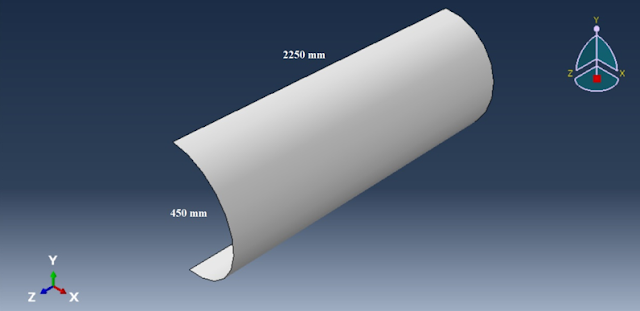
First, a part is created in Abaqus CAE, where a 3-point arc is chosen to draw a half circle with radius 450 mm. Since, the part is selected as 3D shell with extrusion, the length is 2250 mm. We will use symmetry and that’s why, these dimensions are selected to use symmetry boundary conditions about X and Z-axes.

The S4R shell element is chosen with reduced integration for analysis.

Meshing

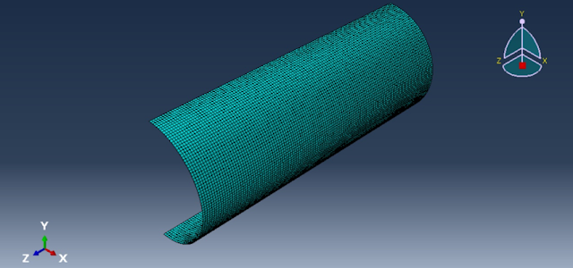
Next, we create the mesh. The mesh size is set to 18 mm, which is twice the size of the shell thickness.

Creating Section

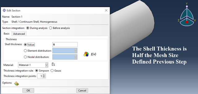
After that, the sections are created. The shell thickness is set 9 mm as per the problem.

Assigning Section

After creating the section, we assign it to the part. Then, we use “Render Shell Thickness” to show the shell thickness.

Creating Partition

A partition is created with 200 mm offset from one of the pipe edges.

Setting Material Properties

For the elastoplastic behaviour, the following material properties are given:

Creating Steps with Loads and Boundary Conditions

In this step, we define the boundary condition (BC) and load. A reference point (RP) is created to fix one end of the pipe. For the RP, a rigid body constraint is defined. Three BCs are generated as follow:

BC-1: for symmetry about X-axis

BC-2: for symmetry about Z-axis

BC-3: for the reference point (RP1), which is fixed along the axes.

Then, a pressure load of magnitude 12.8 MPa is applied inside the pipe.

Results and Discussions: 

Since the model is created with necessary boundary conditions and loads, in this section, we are interested to consider two circumstances.

• Buckling when both pressure and bending are considered

• Buckling when bending is considered without pressure

We apply the static Rik’s approach as a force control. The following figure shows the Von Mises stress when only pressure is applied inside the wall of the pipe.

Buckling when both pressure and bending are considered

At first, we apply a moment of 5x10^10 Nmm at the reference point by creating a new step where Rik’s static algorithm is selected. In this scenario, the pressure is still present inside the pipe. The following figure demonstrates the three steps for the simulation.

The following figure shows two relationship when pressure is present: moment vs arc length and rotation vs arc length. The intersection point between two graphs in the figure is the convergence point for the simulation.

Showing relationships between moment and arc length, and rotation and arc length with pressure

The following plot shows the relation between moment and angular displacement when pressure is present in the pipe.

Buckling when bending is considered without pressure

In this step, we just suppress the load leaving all other conditions same. We are interested to see the effect of the bending only on the buckling rate of the pipe.

Showing 2 steps: no pressure (left), and with angular displacement (right)



The following figure shows two relationship when pressure is absent: moment vs arc length and rotation vs arc length. The intersection point between two graphs in the figure is the convergence point for the simulation.

Showing relationships between moment and arc length, and rotation and arc length without pressure

Moment without pressure (left) and rotation without pressure (right) when arc length is 0.8016 mm

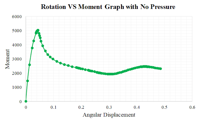
The following plot shows the relation between moment and angular displacement when pressure is absent in the pipe.

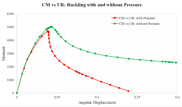
From the following comparison, we see that the buckling is higher when there is no pressure than the buckling with internal pressure.

To learn in detail of FEA, you may visit here.

#VonMisesstress #Buckling #Bending #FiniteElementAnalysis #FEA #Abaqus #ModellingSimulation #Blog #Blogger