Explicit Euler Method to Solve System of ODEs in MATLAB

In this tutorial, I am going to show a simple way to solve system of first order ordinary differential equations (ODE) by using explicit Euler method. Let' say, we have following three first order ODEs.

Here, we have 3 ODEs, 3 dependent variables (x, y, z), and 1 independent variable, t. The initial conditions when time is zero are, x(0) = y(0) = z(0) =1. Our goal is to solve these differential equations with explicit Euler approach and plot the solutions afterwards.

Step 1: Define the Equations

The first step is to define all the differential equations in MATLAB. I did this by using MATLAB function handle, which is shown below.

Step 2: Choose a Numerical Approach 

The next step is to select a numerical method to solve the differential equations. In this example, we will use explicit Euler method. I have created a function to implement the algorithm. The following image shows the application of the explicit Euler method.

Step 3: Call the Function

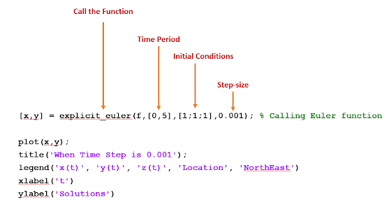
This is the final step where we need to call the function. In the previous step, we have created a function, which we are going to call in this step to solve the equations.

 

So, that's it. We are done with the process, and we can now visualize the solution. I have also attached the MATLAB codes for this problem at the end.

MATLAB Program:

close all;

clc;

format long;

% Defining the three differential equations of the problem

f = @(t,y) [-5*y(1)+5*y(2); 14*y(1)-2*y(2)-y(1)*y(3); -3*y(3)+y(1)*y(2)];

[x,y] = explicit_euler(f,[0,5],[1;1;1],0.001); % Calling Euler function

plot(x,y);

title('When Time Step is 0.001');

legend('x(t)', 'y(t)', 'z(t)', 'Location', 'NorthEast')

xlabel('t')

ylabel('Solutions')

function [x, y] = explicit_euler( f, xRange, y_initial, h )

% This function uses Euler’s explicit method to solve the ODE

% dv/dt=f(t,v); x refers to independent and y refers to dependent variables

% f defines the differential equation of the problem

% xRange = [x1, x2] where the solution is sought on

% y_initial = column vector of initial values for y at x1

% numSteps = number of equally-sized steps to take from x1 to x2

% x = row vector of values of x

% y = matrix whose k-th column is the approximate solution at x(k)

x(1) = xRange(1);

numSteps = ( xRange(2) - xRange(1) ) /h ;

y(:,1) = y_initial(:);

for k = 1 : numSteps

x(k + 1) = x(k) + h; 

y(:,k+1) = y(:,k) + h * f( x(k), y(:,k) );

end

#ExplicitEulerMethod #Matlab #NumericalMethod #Blog #Blogger

Discussion on Numerical Integration Approaches with MATLAB

In this tutorial, we are going to implement four numerical integration schemes in MATLAB. The methods are:

i)   Midpoint Rectangle Rule

ii)  Trapezoidal Rule

iii) Simpson’s 1/3 Rule

iv) Simpson’s 3/8 Rule

Let's say, we would like to integrate the following error function where the upper interval, a is 1.5. At first, we will evaluate the true integral of the error function, and then, we will find the integral numerically with the above methods (i) -(iv).

Finally, we will compare each method with the true value and make some comments based on the deviations if we have any. For each method, we will find out the following parameters:

Here, n refers to the numbers, 1,2,4,8,16, ...,128. I_num is the numerical value of integration, h is the step size, and E is the error, which is the absolute difference between true and numerical results. First, we are going to determine the true value of the error function while integrating from 0 to 1.5. Then, we will apply the corresponding methods and compare the absolute error.

MATLAB Code for Midpoint Rectangle Rule

close all;

clear;

clc;

 

% Defining the error function

f = @(x) (2/sqrt(pi))*exp(-x.^2);

a = 0;

b = 1.5; % Upper integration limit

n = [1 2 4 8 16 32 64 128];

L = length(n);

% Exact integral using MATLAB built-in function

I = integral(f,a,b);

 

fprintf('\n     n          h         I_NUM          E')

 

for j = 1:L

    h(j)=(b-a)/n(j);

   

x_1 = a:h(j):b;

% Using MATLAB built-in command for repeated arrays

x_2 = repelem(x_1(2:end-1),2); 

xh = [a x_2 b];

 

% Numerical integration by mid-point rectangular rule

I_NUM=0;

for i = 1:length(x_1)-1

    I_NUM = I_NUM + f(a  +(i-1/2).*h).*h;

end

 

% Defining the error

E(j) = abs(I-I_NUM(j));

 

fprintf('\n %5.6g %11.6g %12.6g %10.6g', n(j), h(j), I_NUM(j), E(j))

fprintf('\n')

 

end

The following table shows the parameters determined by this approach:

MATLAB Code for Trapezoidal Rule

close all;

clear;

clc;

 

% Defining the error function

f = @(x) (2/sqrt(pi))*exp(-x.^2);

a = 0;

b = 1.5; % Upper integration limit

n = [1 2 4 8 16 32 64 128];

L = length(n);

% Exact integral using MATLAB built-in function

I = integral(f,a,b);

 

fprintf('\n     n          h         I_NUM          E')

 

for j = 1:L

    h(j)=(b-a)/n(j);

% Numerical integration using Trapezoidal rule

I_NUM=0;

for i = 1:n(j)

    I_NUM = I_NUM+(f(a+(i-1).*h) + f(a+i.*h)).*h/2;

end

 

% Defining the error

E(j) = I - I_NUM(j);

 

fprintf('\n %5.6g %11.6g %12.6g %10.6g', n(j), h(j), I_NUM(j), E(j))

fprintf('\n')

end

The following table shows the parameters determined by this approach:

MATLAB Code for Simpson’s 1/3 Rule

close all;

clear;

clc;

 

% Defining the error function

f = @(x) (2/sqrt(pi))*exp(-x.^2);

a = 0;

b = 1.5; % Upper integration limit

n = [1 2 4 8 16 32 64 128];

L = length(n);

% Exact integral using MATLAB built-in function

I = integral(f,a,b);

 

fprintf('\n     n          h         I_NUM          E')

for j = 1:L    

    h(j) = (b-a)/(2*n(j));  

 

% Numerical integration using Simpson’s 1/3 rule

 

I_NUM = 0;

 

for i = 1:n(j)

    I_NUM = I_NUM+(f(a+(2*i-2).*h) + 4*f(a+(2*i-1).*h) + f(a+(2*i).*h)).*h./3;

end

E(j) = abs(I - I_NUM(j));

 

fprintf('\n %5.6g %11.6g %12.6g %10.6g', n(j), h(j), I_NUM(j), E(j))

fprintf('\n')

end

The following table shows the parameters determined by this approach:

MATLAB Code for Simpson’s 3/8 Rule

close all;

clear;

clc;

 

% Defining the error function

f = @(x) (2/sqrt(pi))*exp(-x.^2);

a = 0;

b = 1.5; % Upper integration limit

n = [1 2 4 8 16 32 64 128];

L = length(n);

% Exact integral using MATLAB built-in function

I = integral(f,a,b);

 

fprintf('\n     n          h         I_NUM          E')

for j = 1:L  

h(j) = (b-a)/(3*n(j)); 

 

% Numerical integration using Simpson’s 3/8 rule

I_NUM = 0;

for i=1:n(j)

    I_NUM = I_NUM + (f(a+(3*i-3).*h) + 3*f(a+(3*i-2).*h) + 3*f(a+(3*i-1).*h) + f(a+(3*i).*h))*3.*h/8;

end

 

% Defining the error

E(j) = abs(I - I_NUM(j));

 

fprintf('\n %5.6g %11.6g %12.6g %10.6g', n(j), h(j), I_NUM(j), E(j))

fprintf('\n')

 

end

The following table shows the parameters determined by this approach:

We see from the above comparisons that both Simpson's rules give us a good approximation of the true value, especially when n is greater than 4. For the rectangular approach, the value reaches close to the true value when n is 128. The same is also evident for the trapezoidal rule. So, we can conclude that both the Simpson's rules are more efficient and accurate approaches compared to the rest.

#TrapezoidalRule #SimpsonsRule #Matlab #NumericalIntegration #Blog #Blogger

Stress and Strain Analysis of Linear Finite Elements

In this tutorial, we will use principle of virtual work method to determine the stress and displacement of the nodes of linear one dimensional finite elements. Following figure 1 represents a cantilever beam which is stressed axially. Let's assume the parameters L, A, E, c have the same value of 1 unit for simplicity. Our goal is to compare the finite element results with the exact solutions of a typical cantilever problem.

For this problem, we need to consider two quadratic one dimensional element. So, the displacement is interpolated among the three nodes and has the following form:

Fig.1: Showing one dimensional axially load bar given in the assignment problem.

Fig.2: Showing one dimensional piecewise linear interpolation.

Mathematica Program for Element 1

Clear[x, a0, a1, a2, u1, u2, u3, L]

(*Definition of quadratic form of displacement*)

u = a0 + a1*x + a2*x^2;

eq1 = (u /. x -> 0) - u1;

eq2 = (u /. x -> L/4) - u2;

eq3 = (u /. x -> L/2) - u3;

sol = Solve[{eq1 == 0, eq2 == 0, eq3 == 0}, {a0, a1, a2}];

u = u /. sol[[1]]

N1 = Coefficient[u, u1];

N2 = Coefficient[u, u2];

N3 = Coefficient[u, u3];

(*Shape Functions*)

Nn = {N1, N2, N3}

(*Applied Axial Load*)

p = c*x;

(*Nodal Force Vectors*)

fe = Integrate[Nn*p, {x, 0, L/2}];

c = 1;

L = 1;

fe // MatrixForm

Program Outputs

Displacement Vector for Element 1:

Shape Functions for Element 1:

Nodal Force Vector for Element 1:

Mathematica Program for Element 2

Clear[x, a0, a1, a2, u1, u2, u3, L]

(*Definition of quadratic form of displacement*)

u = a0 + a1*x + a2*x^2;

eq1 = (u /. x -> 0) - u1;

eq2 = (u /. x -> L/4) - u2;

eq3 = (u /. x -> L/2) - u3;

sol = Solve[{eq1 == 0, eq2 == 0, eq3 == 0}, {a0, a1, a2}];

u = u /. sol[[1]]

N1 = Coefficient[u, u1];

N2 = Coefficient[u, u2];

N3 = Coefficient[u, u3];

(*Shape Functions*)

Nn = {N1, N2, N3}

(*Applied Axial Load*)

p = c*(x + L/2);

(*Nodal Force Vectors*)

fe = Integrate[Nn*p, {x, 0, L/2}];

c = 1;

L = 1;

fe // MatrixForm

Program Outputs

Displacement Vector for Element 2

Shape Functions for Element 2

Nodal Force Vector for Element 2

Local Stiffness Matrix for Element 1

Clear[x, a0, a1, a2, u1, u2, u3, L, EA]

(*Definition of quadratic form of displacement*)

u = a0 + a1*x + a2*x^2;

eq1 = (u /. x -> 0) - u1;

eq2 = (u /. x -> L/4) - u2;

eq3 = (u /. x -> L/2) - u3;

sol = Solve[{eq1 == 0, eq2 == 0, eq3 == 0}, {a0, a1, a2}];

u = u /. sol[[1]];

N1 = Coefficient[u, u1];

N2 = Coefficient[u, u2];

N3 = Coefficient[u, u3];

B = {{D[N1, x], D[N2, x], D[N3, x]}};

(*Local Stiffness Matrix*)

K = Integrate[EA*Transpose[B].B, {x, 0, L/2}];

L = 1;

EA = 1;

K // MatrixForm

Program Outputs

Comparison between the Exact and Solution using Four Elements

We know that the exact solution for the axially loaded bar shown in Fig. 1 may be written as,

Where, for the consecutive four elements, we may write the displacement for each element as,

From the assignment problem, the parameter values are,

From the virtual work method, we may write,

The internal virtual work (IVW) may be expressed as,

And, the external virtual work may be presented as,

MATHEMATICA PROGRAM

The following program is written to determine the nodal displacement using the finite element method considering the principle of virtual work. 

Clear[x, a0, a1, a2, u1, u2, u3, L]

(*Definition of quadratic form of displacement*)

u = a0 + a1*x + a2*x^2;

eq1 = (u /. x -> 0) - u1;

eq2 = (u /. x -> L/4) - u2;

eq3 = (u /. x -> L/2) - u3;

sol = Solve[{eq1 == 0, eq2 == 0, eq3 == 0}, {a0, a1, a2}];

u = u /. sol[[1]];

(*Shape Functions*)

N1 = Coefficient[u, u1];

N2 = Coefficient[u, u2];

N3 = Coefficient[u, u3];

Nn = {N1, N2, N3};

B = {{D[N1, x], D[N2, x], D[N3, x]}};

c = 1;

L = 1;

EA = 1;

(*Axial Force on Element 1*)

p1 = c*x;

fe1 = Integrate[Nn*p1, {x, 0, L/2}];

(*Axial Force on Element 2*)

p2 = c*(x + L/2);

fe2 = Integrate[Nn*p2, {x, 0, L/2}];

K1 = Integrate[EA*Transpose[B].B, {x, 0, L/2}];

K2 = Integrate[EA*Transpose[B].B, {x, 0, L/2}];

Ndof = 5;

Ne = 2;

ID1 = {1, 2, 3};

ID2 = {3, 4, 5};

K = ConstantArray[0, {Ndof, Ndof}];

K[[ID1, ID1]] = K1 + K[[ID1, ID1]];

K[[ID2, ID2]] = K2 + K[[ID2, ID2]];

fe = ConstantArray[0, {Ndof, 1}];

fe[[ID1]] = fe1 + fe[[ID1]];

fe[[ID2]] = fe2 + fe[[ID2]];

IDE = {1};

IDN = {2, 3, 4, 5};

KR = Delete[K, IDE];

KR = Delete[Transpose[KR], IDE];

KR = Transpose[KR];

feR = Delete[fe, IDE];

(*Calculation of Nodal Displacements*)

DisR = LinearSolve[KR, feR];

Dis = ConstantArray[0, {Ndof, 1}];

Dis[[IDN]] = DisR + Dis[[IDN]];

Dis // MatrixForm

Program Outputs

So, we see that the exact and finite element solutions are the same.

From the following two plots, we notice that although the nodal displacement is continuous from the FEA result, it is not true for the stress. The stress distribution is indeed discontinuous.

MATHEMATICA PROGRAM FOR COMPARISON

(*Exact Solution*)

uexact = c*L^2/2/EA*x - c/6/EA*x^3;

(*Finite Element Approximation*)

N1 = Piecewise[{{4 x/L, 0 <= x <= L/4}, {4/L (L/2 - x), 

     L/4 <= x <= L/2}}, 0];

N2 = Piecewise[{{4/L (x - L/4), L/4 <= x <= L/2}, {4/L (3 L/4 - x), 

     L/2 <= x <= 3 L/4}}, 0];

N3 = Piecewise[{{4/L (x - L/2), L/2 <= x <= 3 L/4}, {4/L (L - x), 

     3 L/4 <= x <= L}}, 0];

N4 = Piecewise[{{4/L (x - 3 L/4), 3 L/4 <= x <= L}}, 0];

u1 = c*L^3/EA*(47/384);

u2 = c*L^3/EA*(11/48);

u3 = c*L^3/EA*(39/128);

u4 = c*L^3/EA*(1/3);

(*Calculating Nodal Displacement*)

u = u1*N1 + u2*N2 + u3*N3 + u4*N4;

uexactp = uexact /. {c -> 1, EA -> 1, L -> 1}

sigmaexact = D[uexactp, x]

up = u /. {c -> 1, EA -> 1, L -> 1}

sigmap = D[up, x]

(*Plotting to Show the Comparison between Exact and FEA Solution*)

Plot[{uexactp, up}, {x, 0, 1}, 

 AxesLabel -> {"x", "Nodal Displacement"}, 

 PlotLegends -> {"uexact", "u_Finite Element"}]

Plot[{sigmaexact, sigmap}, {x, 0, 1}, AxesLabel -> {"x", "sigma_11"}, 

 PlotLegends -> {"sigma_exact", "sigma_Finite Element"}]

For further information on finite element analysis and Mathematica, readers are encouraged to visit this page.

#FiniteElement #StressStrain #Mathematica #Abaqus #FEA #Blog #Blogger

Some Frequently used Interpolation Tools by MATLAB

Interpolation is a very essential tool in any areas of research these days. Whether you are analyzing your data or deriving equations to represent a system, interpolation plays an immense role in these works. Luckly, MATLAB has some built-in commands for basic data fitting. Not only that, you may also create your own function and use it stand alone or in combination of calling some MATLAB commands. In this article, I am going to discuss three basic techniques for basic data fitting. They are,

• Polynomial Interpolation
• Piecewise Linear Interpolation
• Cubic Spline Interpolation

Polynomial Interpolation: Polynomial interpolation is one of the most basic interpolation tools. The first step would be to learn this technique manually as it would provide us insights into the fundamentals prior to using MATLAB built-in features. The idea is that a polynomial of n degree would pass through all the (n+1) points if we apply the technique of polynomial interpolation. Let us begin with an example to strengthen the concept. 

Let’s say, we have data points: (1, 2.1), (2, 4.6), (3, 5.7) and (4, 9.8). The goal is to fit a polynomial that would pass through all these points. We may consider these points as (x₁, y₁), (x2, y2), (x3, y3), and (x4, y4) where x refers to the horizontal axis and y refers to the vertical axis.

Data points from the example

Now, let's define a general polynomial equation. The following is the n-th order polynomial:



If we extend the general polynomial, it looks like the following as,

And, in matrix form, we may arrange these equations nicely as follows,

For our example problem, we have 4 data points, which means that we will have four equations. The right side vector b is for the vertical (y-axis) data points. The left side nxn matrix is for the horizontal (x-axis) data points. But, there is a question. The horizontal data points are not in a squared matrix, specifically, it is now in 1x4 form; so, how could we represent the data as in a 4x4 matrix for our example? The following figure shows the current configuration:

We can write a simple MATLAB program to make that 4x4 matrix. The following codes will generate a square matrix from a single row matrix.

% Generation of a Polynomial Matrix

x=[1 2 3 4]; % Sample x data points

n = length(x); 

A = zeros(n,n);

 

for i=1:n

% Creating polynomial matrix

for j=1:n

% nth degree polynomial passing through (n-1) points

A(i,j) = x(i).^(j-1);

end

end

disp(A)

After implementing the above program, we will have the following refined equations, which we can solve by Gaussian elimination to find the value of the unknown coefficients, a.

Now, using the Gaussian elimination, the unknown parameters are,

So, the polynomial equation that will pass through all the four points is,

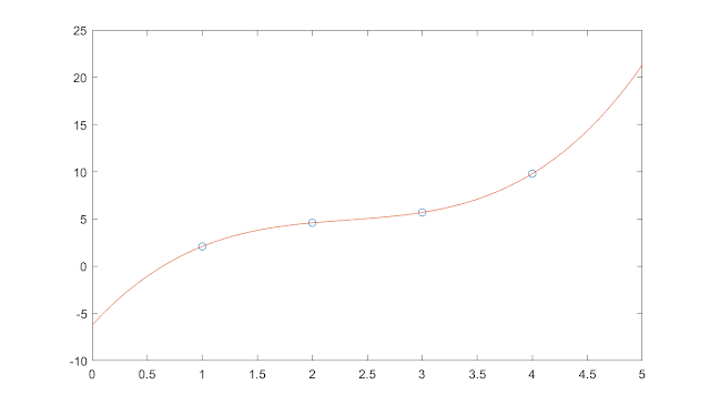
If we plot, the above equation fits and passes through all the points. 

So far, the mathematics behind polynomial interpolation has been discussed. Good news! MATLAB has a built-in polynomial interpolation feature. We can use the feature easily. You can access the built-in function from the command prompt shown as below,

>> x = [1; 2; 3; 4];

>> y =[2.1; 4.6; 5.7; 9.8];

>> polyfit(x,y,3)

ans =

-6.2

12.667

-5.10

0.7333

'polyfit' is the built-in command in MATLAB that uses the same technique shown earlier. 

Piecewise Linear Interpolation: When we have more data points to fit, polynomial interpolation does generate too much oscillations in curve fitting. In this case, we may use the MATLAB built-in command 'interp1' for one dimensional piecewise linear interpolation. For our four data points example, we may write few lines in MATLAB command prompt to access this feature.

>> x1 = [1;2;3;4];

>> y1 =[2.1; 4.6; 5.7; 9.8];

>> xx = 0:0.1:5;

yy = interp1(x1,y1,xx);

plot(x1,y1,'o',xx,yy)

Cubic Spline Interpolation: An improvement to one dimensional piecewise linear interpolation is the cubic spline interpolation. We may use the MATLAB built-in command 'spline' for it. For our four data points example, we may write few lines in MATLAB command prompt to access this feature.

>> x1 = [1;2;3;4];

>> y1 =[2.1; 4.6; 5.7; 9.8];

>> xx = 0:0.1:5;

yy = spline(x1,y1,xx);

plot(x1,y1,'o',xx,yy)

#Interpolation #PiecewiseLinear #CubicSpline #Matlab #Polynomial #Blog #Blogger