Welcome to the World of Modelling and Simulation

What is Modelling?

This blog is all about system dynamics modelling and simulation applied in the engineering field, especially mechanical, electrical, and ...

A MATLAB Program to Implement the Jacobi Iteration

A MATLAB Program to Implement Jacobi Iteration to Solve System of Linear Equations:

The following MATLAB codes uses Jacobi iteration formula to solve any system of linear equations where the coefficient matrix is diagonally dominant to achieve desired convergence.

%-----------------------------------------------------------------%
function [x, rel_error] = jacobimethod(A, b, x0, tol, iteration)

% Inputs: A - Coefficient matrix
%         b - Input matrix
%       tol - Defining tolerance for solution
% iteration - Number of iterations

% Outputs: x - Solutions
%  rel_error - Relative error

D = diag(diag(A));   % Making coefficient matrix diagonal
R = A - D;           % Construction of another matrix "R"
N = 1;               % iteration counter
x = x0;
rel_error = tol * 2; % norm(x - x0)/norm(x);

% Implementation of Jacobi method to solve Ax = b
while (rel_error>tol && N <= iteration)
   
    xprev = x;   
    x = inv(D)*(b - R*xprev);
    rel_error = norm(x - xprev)/norm(x);

    Z1=x(1);
    disp(Z1);
    Z2=x(10);
    disp(Z2);
    Z3=x(16);
    disp(Z3);
   
    fprintf('\n Iteration %i: Relative error =%d ',N, rel_error)   
    N = N + 1;       
end
%----------------------------------------------------------------%

Now, define your input matrices in the MATLAB command window and use the above developed function to compute Jacobi iteration.

MATLAB Command Prompt:

>> A = [-2 1 0 0 0 0 0 0 0 0 0 0 0 0 0 0;
    1 -2 1 0 0 0 0 0 0 0 0 0 0 0 0 0;
    0 1 -2 1 0 0 0 0 0 0 0 0 0 0 0 0;
    0 0 1 -2 1 0 0 0 0 0 0 0 0 0 0 0;
    0 0 0 1 -2 1 0 0 0 0 0 0 0 0 0 0;
    0 0 0 0 1 -2 1 0 0 0 0 0 0 0 0 0;
    0 0 0 0 0 1 -2 1 0 0 0 0 0 0 0 0;
    0 0 0 0 0 0 1 -2 1 0 0 0 0 0 0 0;
    0 0 0 0 0 0 0 1 -2 1 0 0 0 0 0 0;
    0 0 0 0 0 0 0 0 1 -2 1 0 0 0 0 0;
    0 0 0 0 0 0 0 0 0 1 -2 1 0 0 0 0;
    0 0 0 0 0 0 0 0 0 0 1 -2 1 0 0 0;
    0 0 0 0 0 0 0 0 0 0 0 1 -2 1 0 0;
    0 0 0 0 0 0 0 0 0 0 0 0 1 -2 1 0;
    0 0 0 0 0 0 0 0 0 0 0 0 0 1 -2 1;
    0 0 0 0 0 0 0 0 0 0 0 0 0 0 1 -2];

>> b = [-1; -2; -2; -2; -2; -2; -2; -2; -2; -2; -2; -2; -2; -2; -2; 1];

>> x0 = [0; 0; 0; 0; 0; 0; 0; 0; 0; 0; 0; 0; 0; 0; 0; 0];

>> tol=10^-5;

>> iteration=350;

>> jacobimethod(A, b, x0, tol, iteration)


ans =

   14.8499
   28.7009
   40.5541
   50.4104
   58.2708
   64.1360
   68.0066
   69.8830
   69.7653
   67.6537
   63.5477
   57.4473
   49.3516
   39.2600
   27.1715
   13.0852

A MATLAB Program to Determine the Roots of Equation by Secant method

Problem: Solve the following problem by Secant Method.

f(x) = x - 2e^-x

Determine the roots of the above function where x1 = 0 and x2 = 1.


Solution: The following MATLAB program solves this problem.

% Definition of a function "secantmethod" to solve equation by Secant Method

function [x,ea] = secantmethod(X,X0,etol)

format long;

% Input: X=0, etol=Tolerance definition for error
% Output x=Solution of equation, ea=Calculated error in loop

% Program Initialization

% Iterative Calculations

while (1)
   
    % Implementation of Secant Method
         
    solution = X-((X-(2*exp(-X)))*(X0-X))/((X0-(2*exp(-X0)))-(X-(2*exp(-X))));    
   
    solutionprevious=X;
    X0=X;
    X=solution;
                 
if (solution-solutionprevious)~=0          % Approximate percent relative error
                                
   ea=abs((solution - solutionprevious)/solution)*100;
      
end

if ea<=etol                 
  
    break,               
end

%x0=solutionprevious;
x = solution;

%disp(x0);
disp(x);

end

% Display of output parameters

disp(x);                     

disp(ea);

%disp(solution-(0.1*abs(ea)*solution));

end


Program Outputs:

>> secantmethod(1,0,1e-10)

   0.883298154248460

   0.851584208519236

   0.852612692886131

   0.852605503703827

   0.852605502013723

   0.852605502013723

     3.125167797776517e-13


ans =

   0.852605502013723


#SecantMethod

My First Code in Python: Adding all Prime Numbers

As Python programming is highly hyped now-a-days and a frequent buzzword in machine learning and AI communities, I have decided to get myself familiar in this area. As I learn and decipher the Python coding day-by-day, I will be more than happy to share my coding in this blog. Here is my first program in Python - to develop a logic that adds all prime numbers between 0 and a given number.

We know that a prime number is an integer, which is greater than one and which is only divisible by one and itself. The following shows an algorithm that adds all prime numbers between 0 and a given number.

Development of an algorithm to add all prime numbers between 0 to n

I. First, we define the lower and upper number to initialize the program. For example, we set the lower number 0 and upper number 10; and we are interested to find the summation of prime numbers in this range.
II. Prime number is greater than one, so our logic begins that it must be greater than one. Therefore, we begin with number 2 and list all the numbers in our range.
III. Since, prime numbers are divisible only by itself and one; we create a loop, which confirms the prime numbers, and display them. We implement this by checking if the remainder of the number is zero or not. If the remainder is zero, then it is not a prime number.
IV. If the remainder of the number is not zero, then it is a prime number.
V. Display the prime numbers in the defined range and group the numbers in a list or array.
VI. Finally, we add all the prime numbers in the list.

The following Python code is developed based on the above algorithm, which displays all the prime numbers in a given range and add those numbers:


lower = 0

upper = 10     #Defining the range

sum1 = 0       #Setting Summation of prime numbers to zero

print("Prime numbers between", lower, "and", upper, "are:")

for num in range(lower, upper + 1):

   if num > 1:                 #Prime number is greater than 1

       for i in range(2, num):

           if (num % i) == 0:  #Calculates & checks remainder of division

               break
       else:
         
           print(num)  # Displays prime numbers
         
           sum1 += num
         
print(sum1)


Program Outputs:

Prime numbers between 0 and 10 are:
2
3
5
7
17


#Blog #Blogger #Python #PrimeNumber #Algorithm

Looking for an Industrial Partner to Implement a Lemon Shaped Guide to Minimize Rubbing

A NOVEL LEMON SHAPED GUIDE TO MINIMIZE EXCESSIVE RUBBING IN ROTATING MACHINES

In industries, rotating machines are widely used, because rotation offers a great way to transfer power from one point to another and convert motion to different planes by gears, belts, shaft etc. A rotating machine typically includes a rotor, bearings and a support structure. There are critical relations among these components where each component of a system influences the overall dynamic behavior of a machine. For example, rotor-to-guide rub degrades a mechanical system over the years and may even cause fatal accidents earlier. It is, therefore, paramount in industries, to run rotating machines, operating at high speeds smoothly and reliably. The primary reasons of rubbing between a rotor and a guide are due to a manufacturing error, excessive imbalance, misalignment, bearing wear, smaller radial clearance between the rotating shaft and casing, bad assembly, etc. Rub occurs in rotor casing, seals, unlubricated journal bearings, loose rotor guide attached to restrict a large deflection. The problem is prevalent in the industry and demonstrated in several literatures. To deal with this problem, the industry has already been using circular shaped guide to minimize excessive vibration between a rotor and a stator. Although, the circular shaped guide may reduce the vibration, but the rub, between rotor and guide, may still be present, which may lead to the permanent damage of a mechanical system. The lemon shaped guide is not only effective in minimizing rubbing between rotor and stator, but also it suppresses the excessive vibration similar to the circular shaped guide.

The following video shows an experiment on how to minimize rubbing between a rotor and a guide that typically happens in a high speed rotating machine with a newly developed lemon shaped bearing or guide. We see here as the speed goes high, the system enters into its resonance frequency where it vibrates excessively. The lemon/elliptical shaped guide helps prevent the excessive rubbing while the rotor-bearing assembly is in the natural frequency zone. It has been found from our research that the lemon shaped guide minimizes rubbing better than the circular shaped guide where there the rotational speed is very high (https://doi.org/10.1115/1.4043817). 


The next video shows an experiment on how to minimize rubbing between a rotor and a guide that typically happens in a high speed rotating machine with a circular bearing or guide. This is a traditional approach, which has been in operation in industries for long. We see in the video, as the speed goes high, the system enters into its resonance frequency where it vibrates excessively. The circular guide helps prevent the excessive vibration while the rotor-bearing assembly is in the natural frequency zone. However, if we notice carefully, the rubbing is still present between the rotor and guide, which deteriorates the system gradually.


A US provisional utility patent (US Patent App. 62/956,833) has already been filed for this design. I am looking for industrial partners or investors if they are interested in investing this product.

Learning Mathematica, Lesson 1: Plotting a Function

This is the very first lesson or tutorial on Mathematica. As I am in the process of learning this tool, I will gradually post more articles on this, ranging from basic to advanced level problems. So, the first question is, what is Mathematica? It is simply a tool for computing, but it has an advantage that the symbolic expression is much user-friendly and more interactive than MATLAB.

Although, MATLAB is a much bigger platform than Mathematica, because MATLAB has numerous toolboxes and libraries that are designed for specific fields. Nevertheless, Mathematica, a product from Wolfram Research, is great for symbolic and interactive computing with a very neat interface. You may try it for free here just to see its environment. Let's start, how Mathematica looks like. After you install it (which isn't complex, it's pretty straightforward, if you just follow the instructions), click on your desktop shortcut and it will look like the following:

how Mathematica looks like

Then, you need to click on the "Documentations" to proceed which will bring the following:

how Mathematica looks like

Now, if you like to start writing you very first code on Mathematica, then click File, and select Notebook.

how Mathematica looks like

Now, write you first code here, and execute it. Let's say, we like to plot a function which looks as follows,

plotting a function in Mathematica

To execute the program above, you need to click on Evaluation and then, select Evaluate Notebook. The variable X varies from 0 to 5.


#Mathematica #Matlab #NoteBook #MatlabvsMathematica #Blog #Blogger

A SIMULINK Model to Solve a Simple Shaft-Disk Dynamics Problem

The following figure 1 represents pretty simple model where two circular disks of inertia J1 and J2 are mentioned. Torque (T) is applied to the disk 1. The shaft has its own stiffness which is K. 

two disks are connected by a shaft
Fig.1: Showing a very simple model where two disks are connected by a shaft and torque is applied to one of them.


At first, let's find the state variables for this problem and then write the state equations.

State Variables and State Equations:

State variables


State equations


Next, we assume the following key parameters,

Initial Conditions:

Initial conditions


Parameter Values:

J1 = 100, J2 = 100, K = 100, and T = 10000. (All values are considered unitless for simplicity)

The SIMULINK model is formed by implementing the state equations. And, the above parameter values are considered. The following simulation results are for the acceleration, velocity and position of the disks which are essentially the outputs from the SIMULINK block diagram.

SIMULINK model of shaft-disk system

Fig.2: SIMULINK model of the shaft-disk system.


Showings the results of angular acceleration, velocity and displacement respectively of disk 1
Fig.3: Showings the results of angular acceleration, velocity and displacement respectively of disk 1.


angular acceleration, velocity and displacement respectively of disk 2
Fig.4: Showings the results of angular acceleration, velocity and displacement respectively of disk 2.


#Simulink #Matlab #ShaftDisk #BlockDiagram #Blog #Blogger

Theory of Energy Conversion in Wind Turbine

In wind turbine, the wind energy is converted to first mechanical energy, and then this energy is converted to electrical energy. Damping is an essential part for a generator. However, it is not the key factor for energy conversion. If there were no damping or loss, we would have 100% efficient conversion. This is not possible in real life, as we would have certain losses during the energy conversion process. These losses are represented by non-conservative forces, such as friction, viscous damping etc. which are the essential parts to be considered in the energy conversion process. I want to show the fundamentals behind energy conversion in DC motor.

DC motor converts electrical energy (input voltage) to mechanical energy (shaft rotation). This electromechanical conversion involves Faraday’s law of induction and Ampere’s law for force generated on the conductor moving in a magnetic field. In ideal situation, the torque (T) developed on the motor shaft is proportional to the input current (I) and the induced electromotive force (EMF) (V) or back EMF is proportional to the speed (W) of the motor. This can be expressed as [1];

T = K1 I ..........................................................(1)

V = K2 W .......................................................(2)

Where, K1 and K2 are the proportionality constant.
The electrical power (Pe) input to the motor is the product of the induced EMF and current.

Pe = VI = K2 W T / K1  ..................................(3)

And, the mechanical power output (Pm) is the product of the speed of the motor and torque.

Pm = T W .......................................................(4)

Now, by comparing equation (3) and (4), the following relation is obtained.

Pe = (K2 /K1) Pm  ...........................................(5)

From Ohm’s law, it is known that,

E - V = I R  ..................................................(6)

Where, E is the input voltage to the motor, and R is the resistance of the motor armature.
Moreover, we also know that torque produced at the motor shaft is equal to the product of the inertia of the load (J) and rate of change of angular velocity or angular acceleration.

T = J (dW/dt)  .............................................(7)

Now, from equations (1), (6) and (7), it is found that

J (dW/dt) = K1 I = K1 / R (E - V)  ...........................................(8)

Using equation (2) further, the following expression can be established.

dW/dt = (K1 K2 / J R) W + (K1 / J R) E  ..................................(9)

The above equation refers to the first order linear differential equation model where ‘W’ represents the state of the system and ‘E’ is the external control input. This first order equation is good enough to predict the output speed of the motor. However, in terms of measuring the position’ it is necessary to add the following equation.

W = dθ / dt  ...........................................................................(10)

Where θ is the output position of the DC motor and refers to another state of the system. Therefore, the model has one control input and two state variables (position and velocity).

By the above mathematical analysis, I want to specify, that the electrical energy is converted to mechanical energy by a gyrator which has a constant ratio K. Here, resistance of the armature is the energy loss during the conversion of electrical to mechanical energy which is also mechanical equivalence of a damper. A damper not only signifies the energy dissipation/loss from a system, but also helps to make a system stable by removing oscillations.


Reference
[1] Control system design : an introduction to state-space methods / Bernard Friedland.—Dover ed.               

Some Remarks on Forces at Contacts in Light of Bond Graph

So, you have already searched something related to "Contact Forces", and found this page. I welcome you to explore my perceptions behind the fundamental concept of contact forces which might satiate your query.

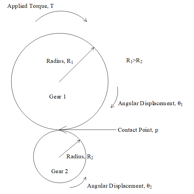
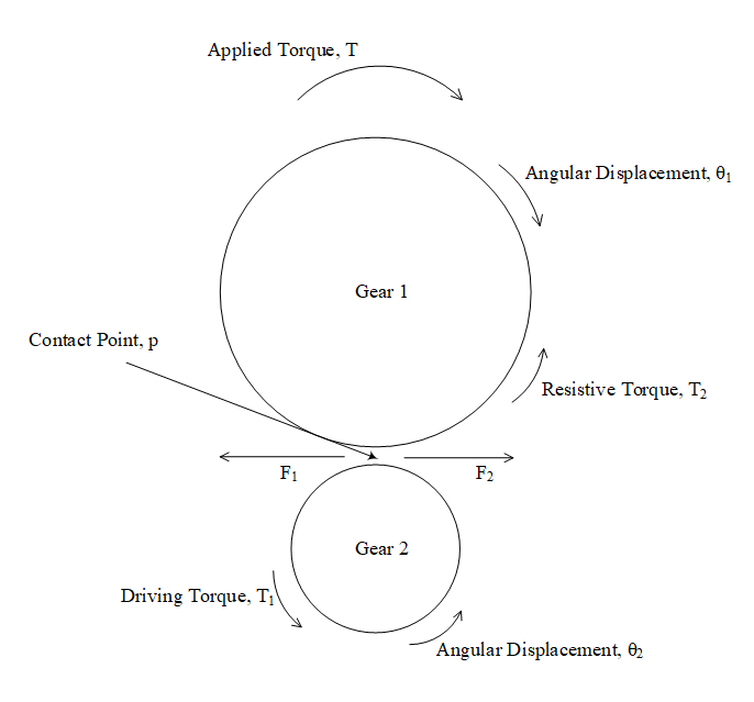
Figure 1 shows a single stage gear train. Torque T is applied on gear 1 which is further driving gear 2. The driver gear is the gear 1 and the driven gear is the gear 2. Here, I will try to explain the mechanics behind this gear mechanism. Figure 2 represents the torques and forces are acting on both of the gears. Gear 1 applies a force F1 which is the actual driving force to rotate the gear 2. This force F1 multiplied with the radius of the gear 2 generates eventually the driving torque T1. According to Newton’s third law, the force F1 applied by gear 1 on gear 2 will be equal and opposite to the force F2 which is the force applied by gear 2 on gear 1. The force F2 similarly generates a torque T2 on gear 1 by multiplication with gear 1 radius, but this torque is the resistive torque for gear 1 as the direction is opposite to the applied torque T. For two mating gears, their directions of angular displacements are opposite to one another, and if I am not wrong, this is physical in real life. For example, in figure 2, direction of angular displacement of gear 1 is clockwise whereas the direction of angular displacement of gear 2 is anti-clockwise.

single stage gear
Figure 1: A single stage gear train.


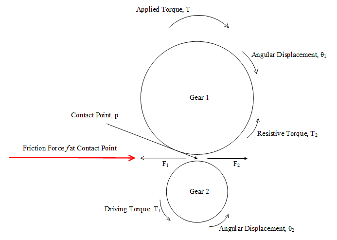
Now, the question arises what is the type of the force F acting between the mating gears? Forces may be divided primarily as conservative and non-conservative forces. If it is conservative force, then the input and output energy must be balanced and the efficiency of the process is 100% which seems ideal. Now, if it is non-conservative force, then there would be energy dissipation from the system and work done by the non-conservative force on gear 2 is negative. Friction force is one of the common non-conservative forces that we experience in our daily life. My intuition in this regard is that this friction force cannot be the driving force for gear 2. The term “Driving Force”, by which, I mean the force helps to rotate gear 2. I will explain my point of view shortly, but before that let us have a look in figure 3 where the presence of the friction is considered. The nature of friction force is to oppose the motion of a moving body and in figure 3 this force acts opposite to the direction of rotation for both of the gears. In figure 3, there are also conservative forces (F1, F2) acting at the contact point p. What if there is only friction force acting at the contact? Then both of the gears would rotate in the same direction viz. clockwise in figure 3. But this is not physical in gear transmission. There have to be the presence of conservative forces with the friction as well. 
FBD of gear train system
Figure 2: Free body diagram of the gear train system.


Now, I would like to explain the role of friction in both sliding and rolling motion. Figure 4 shows a sliding block on both horizontal and inclined planes. In figure 4, F is the applied force on the block which has mass M. While sliding on both the planes a frictional force f is acting between the block and the surface tries to resist the sliding motion of the block. And, the direction of friction is opposite to the direction of translational velocity of the block and it is true for every sliding motion.

Friction force at contact point
Figure 3: Friction force acting at the contact point between gears.


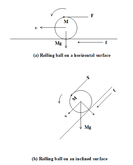
The picture is different in case of rolling motion. Following figure 5, represents a ball rolling on horizontal plane as well as inclined plane. In this case, the friction force acts in the direction of the C.G. translational velocity of the ball. There is no sliding, and that is why, both the directions are same, however, this friction force tries to resist the rotation of the ball. And, eventually the friction force creates a torque which is acting opposite to the applied torque. Here, friction force helps to keep the rolling motion of the body and it is not the driving force. If it were the driving force, then the conservation of energy law would have been violated. Friction might be called driving force in a sense that it helps maintaining rolling motion of the wheel and if there were no friction then the wheel would have been sliding. We see the sliding occurs if a car tries to run over the black ice.

 
Sliding blocks


Figure 4: Sliding blocks on horizontal (a) and inclined (b) planes.


In previous figure 2, the force F is not the friction force, and the way, I considered this force is proportional to the relative tangential displacements of the mating gears. I added a constraint for this force and why I did this, will be enlightened in the next passages.

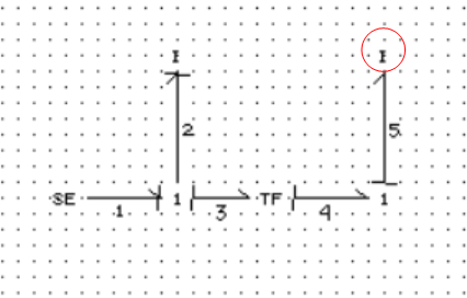
Figure 6 shows the bond graph model of the previous single stage gear train pictured in both figure 1 and 2. There is a special reason to show the bond graph model here although it could simply be done by applying Newton's law. In figure 6, the inertia of the gear 2 is derivative causal, and it is no more acting as a restoring element. It does not create a state of the system. Apparently, the model seems okay, but there is an inherent flaw in the model which does not make the model physical. The natural causality of inertial element is to take effort from the source to generate flow and the relationship is maintained by integration. But, if it is forced to acquire opposite causality, the relationship is governed by differentiation. To overcome this scenario, something has to be present to avoid this derivative causality. We say that the force F1 in figure 2 is the driving force for gear 2 but, how the force is generated? The answer to this question is due the contact between the mating gears. 
Rolling ball
Figure 5: Rolling ball on horizontal (a) and inclined (b) planes.


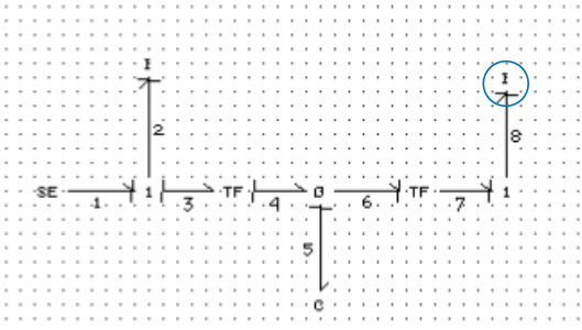
So, gear 1 pushes gear 2 to rotate and according to Newton, gear 2 will try to resist and gives back reaction force. For this to be happened, there should have a medium to transfer the effort from gear 1 to gear 2. And, this medium may be modelled by a compliant element. It should be noted also that this compliant element does not represent contact deformation as it is not considered here. Although, in reality, there is eventually be microscopic deformation between mating gears, but for the case considered here this may be safely ignored. Figure 7 shows the compliant element C which integrates the tangential velocities of the mating gears and the force generated at the contact is proportional to the relative tangential displacements of the mating gears. The tangential velocity at the contact point is obtained by multiplying angular velocity with the radius of the gear and this is performed in the bond graph by TF elements.
Bond graph model of gear train
Figure 6: Bond graph model of the gear train in figure 2 (Derivative Causality).


Newton stated in his third law of motion that every action has an equal and opposite reaction. This is universally true and there is no doubt on this law. So, for an action on a body, according to this law there would be same and opposite reaction which means, Fa = -Fr
Bond graph model of gear train
Figure 7: Bond graph model of the gear train in figure 2 (Integral Causality).


Where, Fa is the action force on a body and Fr is the reaction force by the body. But, the reaction force is created because of the contact or impact, and if we ignore the fact of force transmission between the contacting bodies we would have rigid mass coupling which again imposes derivative causality.