Welcome to the World of Modelling and Simulation

What is Modelling?

This blog is all about system dynamics modelling and simulation applied in the engineering field, especially mechanical, electrical, and ...

A SIMULINK Model for Understanding Encoding and Decoding

Encoders and Decoders

Optical encoders can be classified in two ways:
  • Absolute Encoder
  • Relative/Incremental Encoder
Encoders may have linear or rotary configurations. However, the rotary encoders are common in industry. In absolute encoder, a unique digital word corresponds to each rotational position of the shaft whereas in incremental encoder, by producing digital pulses while the shaft rotates measure the relative displacement of the shaft [1].
In this lab, Incremental encoder is studied and implemented. Incremental encoders are simple in construction and measurement as well.

Objectives
1. To develop a MATLAB program which decodes the input data streams “idatal8” given in the lab materials.
2. Then translating the written MATLAB code into a SIMULINK program.
3. Verification of the decoders by experiment comparing with the built-in decoders in the DC motor kit.

Objective 1
A MATLAB program is developed to decode the input data file “idatal8”. The steps and explanation of the commands are given as notes to the respective lines in the program. The entire program is given below which is based on the decoding logic given in table 1:


Table 1: Decoding of Optical Encoder Signal for Position Measurement [2]
Trigger
Other Channel
Motion Count
A rising (0 to 1)
B high (1)
-1
A rising (0 to 1)
B low (0)
+1
B rising (0 to 1)
A high (1)
+1
B rising (0 to 1)
A low (0)
-1
A falling (1 to 0)
B high (1)
+1
A falling (1 to 0)
B low (0)
-1
B falling (1 to 0)
A high (1)
-1
B falling (1 to 0)
A low (0)
+1


MATLAB Program for Decoding Input Data Streams

close all;

clear all;
format long;

idatal8                         % Running the input data streams

t=1:179;                        % Total Sample    

A=digdata(1,1:179);             % Splitting the "digdata" into two workspaces
B=digdata(2,1:179);

j=1;

for i=1:178;                    % logic created for decoding input data
   
   sum=0;
   
   p=A(1,j);
   q=B(1,j);
   r=A(1,j+1);
   s=B(1,j+1);
    
        if r>p && q==0          % A rising & B low
            
        count=1;
            
        elseif p==1 && s>q      % A high & B rising
        
        count=1;
        
        elseif r<p && q==1      % A falling & B high
        
        count=1;
        
        elseif p==0 && s<q      % A low & B falling
        
        count=1;   
        
        elseif p==0 && s>q      % A low & B rising
            
        count=-1; 
            
        elseif r>p && q==1      % A rising & B high
                 
        count=-1; 
                 
        elseif p==1 && s<q      % A high & B falling
                     
        count=-1;
                     
        elseif r<p && q==0      % A falling & B low             
        
  count=-1;
                                   
        else
            
        count=0;
        
        end  
        
        sum=sum+count;
                                
        X(1,j)=sum;             % Representing motion after decoding
                           
        j=j+1;
        
       
 end
                

figure(1)

subplot (211),plot(t,A,'b'),grid
title('Sequence of Pulses vs Quadrature Signals')
ylabel ('Waveform from Channel A'),xlabel('Pulse Sequences')
subplot (212),plot(t,B,'r'),grid
title('Sequence of Pulses vs Quadrature Signals')
ylabel ('Waveform from Channel B'),xlabel('Pulse Sequences')


figure(2)                       % Decoded Motion

t1=1:178;
plot(t1,X,'b'),grid
title('Forward & Reverse Motion')
ylabel ('Waveform'),xlabel('Motion Counts')


Following figure 1 shows the waveform from channel A and B plotted separately obtained from the data file ‘idatal8’. Figure 2 represents the motion count after decoding the input data streams which eventually dictate the forward and reverse direction by the program algorithm. This figure also highlights the fast and slow sequences of the counts.
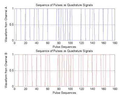
signals from channel A and B


Figure 1: Showing the signals from channel A and B from input data streams ‘idatal8’.

decoded signal from input data streams


Figure 2: Showing the decoded signal from input data streams ‘idatal8’ representing motion.


Objective 2
An incremental or quadrature encoder provides two bit signal. Each signal comes from each of the receivers (channel A and B). These two input streams are offset by ¼ of one of the light or dark bands. For an incremental encoder, the will be four discrete positions for each pulse. These positions are (0,0), (1,0), (1,1) and (0,1). Depending on these 4 distinct positions, the direction of rotation of the motor may be determined by the following table.

Table 2: Direction of Motion Assessment


Forward Motion

Channel A

0          1          1          0          0          1          1          0...................  

Channel B

0          0          1          1          0          0          1          1...................

Backward Motion

Channel A

1          0          0          1          1          0          0          1.................. 

Channel B

0          0          1          1          0          0          1          1..................


A SIMULINK model is created to understanding the position and velocity counting mechanisms of the encoder which is connected to the “DC Motor Kit”. Following figure 3 shows the simple model for the experiment. In the experiment, attempts are taken to measure the resolution of the physical encoder. For this, first the total number of discrete positions is counted for one revolution. For one revolution, there are 7820 distinct points and number of bands or slots on the disk is 1955 (7820/4). For one revolution, the encoder count decreases from 0 to -3950 and then increases to -80 and based on this information the 7820 discrete points are estimated. This calculation might vary, but would provide some insights into position measurement. So, the resolution of the experimental encoder is 0.04º (360/7820) approximately. For each positive or negative counts, there will be a change of position of the motor around 0.04º that the encoder measures.
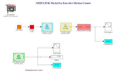
SIMULINK model for encoding decoding

Figure 3: A SIMULINK model for understanding encoding and decoding.

Objective 3
In this part, the algorithm developed earlier in Objective-1 will be verified. For this, the encoder total counts for a single rotation is gathered and stored in the workspace. A truncated data table is provided below to show the trend of the encoder counts.

Table 3: Encoder Reading Pattern from the Experiment

   -1469
-1467
-1465
-1463
-1461
-1459
-1457
-1455
-1453
-1451


Data Truncated


-1701
-1703
-1705
-1707
-1709
-1711
-1713
-1715
-1716
-1718


To verify the MATLAB program, the similar program with some modifications is done which decodes the above data streams. The program for the physical encoder decoding is given below:

MATLAB Program for Decoding Physical Encoder Counts

close all;
clear all;
format long;

inputdatastreams                        % Running data file

t=(1:2707)';
A=counts;             

j=1; 
for i=1:2707;                       
        sum=0;
        p=A(j,1);
        q=A(j+1,1);        
        if q>p                          % Decoding logics            
        count=-1;                
        elseif q<p            
        count=1;                                      
        else            
        count=0;                      
        end          
        sum=sum+count;                            
        X(j,1)=sum;                     % Stores positive/negative counts
                             
        j=j+1;    
end
                
figure(1)                       

plot(t,X,'b'),grid
title('Forward & Reverse Motion')
ylabel ('Waveform'),xlabel('Motion Counts')

Figure 4 shows the decoded signals from the encoder. From the figure, it is observed that the data streams have forward motion, reverse motion, fast and slow rate with the increase of time.

decoded signal from encoder

Figure 4: Showing the decoded signal from encoder data streams.

References
[1] David G. Alciatore, Michael B. Histand, Introduction to Mechatronics and Measurement Systems-fourth edition, The McGraw-Hill Companies, Inc., 2012.
[2] Dr. Jeff Pieper, ENME 560 (Mechatronics Design Laboratory), Lab-05 Manual, 2006.


#Encoder #Decoder #IncrementalEncoder #DataStream #SIMULINK #Blog #Blogger

A MATLAB Algorithm for a Pentadiagonal Matrix

Problem Statement: Develop a computer algorithm for the pentadiagonal matrix with band of b and solve following equations as well.

pentadiagonal matrix

MATLAB Program to Solve a Pentadiagonal Matrix with a band b:

% A function to solve equations which coefficients have form of penta
% diagonal matrix with band b
 
function x=penta_diagonal(A,b)
 
[M,N]=size(A);
% Dimension checking
 
if M~=N
    
    error('Matrix must be square');
    
end
 
if length(b)~=M
    
    error('Matrix and vector must have the same number of rows');
    
end
 
x=zeros(N,1);
    
 
if A==A'    % Matrix symmetry checking
    
    % Band Extractions
    
    d=diag(A);
    f=diag(A,1);
    e=diag(A,2);
    
    disp(d);
    disp(f);
    disp(e);
        
    alpha=zeros(N,1);
    gamma=zeros(N-1,1);
    delta=zeros(N-2,1);
    c=zeros(N,1);
    z=zeros(N,1);
    
    % Factor A=LDL'
    
    alpha(1)=d(1);
    gamma(1)=f(1)/alpha(1);
    delta(1)=e(1)/alpha(1);
    
    alpha(2)=d(2)-f(1)*gamma(1);
    gamma(2)=(f(2)-e(1)*gamma(1))/alpha(2);
    delta(2)=e(2)/alpha(2);
    
    for k=3:N-2
        
        alpha(k)=d(k)-e(k-2)*delta(k-2)-alpha(k-1)*gamma(k-1)^2;
        gamma(k)=(f(k)-e(k-1)*gamma(k-1))/alpha(k);
        delta(k)=e(k)/alpha(k);
    end
    
    alpha(N-1)=d(N-1)-e(N-3)*delta(N-3)-alpha(N-2)*gamma(N-2)^2;
    gamma(N-1)=(f(N-1)-e(N-2)*gamma(N-2))/alpha(N-1);
    alpha(N)=d(N)-e(N-2)*delta(N-2)-alpha(N-1)*gamma(N-1)^2;
    
    % Updating Lx=b, Dc=z
    
    z(1)=b(1);
    z(2)=b(2)-gamma(1)*z(1);
    
    for k=3:N
        z(k)=b(k)-gamma(k-1)*z(k-1)-delta(k-2)*z(k-2);
    end
    
    c=z./alpha;
        
    % Back Substitution L'x=c
    
    x(N)=c(N);
    x(N-1)=c(N-1)-gamma(N-1)*x(N);
    
    for k=N-2:-1:1
        
        x(k)=c(k)-gamma(k)*x(k+1)-delta(k)*x(k+2);
    end  
   
end
 
x;
end


Program Outputs:

ans =

   0.673740053050398
  -1.021220159151194
   1.389920424403183
  -1.148541114058356
   2.055702917771884
  -2.018567639257295

A Modified Thomas Algorithm by MATLAB Codes

Modified Thomas Algorithm: For special matrices such as tridiagonal matrix, the Thomas algorithm may be applied. The given matrix in the question is not in tri-diagonal format. So, in the following program, the matrix is made tridiagonal by taking coefficients of the upper and lower triangles to the right side of the equation and then the algorithm is implemented. The initial guesses for the solutions are assumed which is corrected iteratively in the program. This means the initial guesses are substituted to the right hand side variables and then by Thomas algorithm new solutions are obtained which then again are considered as initial values based on the no of iterations and error limit. The process is simply iterative. The matrix in the following is not convergent by Thomas algorithm.


System of Algebraic Equations


A MATLAB Program for Modified Thomas Algorithm

% Modified Thomas Algorithm to solve system of equations iteratively
 
a=[1 -1 4 0 2 9; 0 5 -2 7 8 4; 1 0 5 7 3 -2; 6 -1 2 3 0 8; -4 2 0 5 -5 3; 0 7 -1 5 4 -2]; % Given Matrix
 
b=[19; 2; 13; -7; -9; 2]; % System input
 
a1=[1 -1 0 0 0 0; 0 5 -2 0 0 0; 0 0 5 7 0 0; 0 0 2 3 0 0; 0 0 0 5 -5 3; 0 0 0 0 4 -2]; % Making original 
                                 % matrix into tridiagonal form by taking coefficients to the right side
 
c=1;
 
N=4; % No of iterations
 
e=[0.1; 0.1; 0.1; 0.1; 0.1; 0.1]; % Error tolerance
 
x(1,1)=0; x(2,1)=0; x(3,1)=0; x(4,1)=0; x(5,1)=0; x(6,1)=0; % Assuming initial solutions to continue 
                    % algorithm as the right hand side of equation contains variables with coefficient
 
 
while(c<N)
    
    x0=[x(1,1); x(2,1); x(3,1); x(4,1); x(5,1); x(6,1)];         % Initial solution
 
b1=[19-(4*x(3,1))-(2*x(5,1))-(9*x(6,1));                % Modified input matrix 
    2-(7*x(4,1))-(8*x(5,1))-(4*x(6,1));
    13-x(1,1)-(3*x(5,1))+(2*x(6,1));
    -7-(6*x(1,1))+x(2,1)-(8*x(6,1));
    -9+(4*x(1,1))-(2*x(2,1));
    2-(7*x(2,1))+x(3,1)-(5*x(4,1))];
 
%disp(b1);
 
for i=2:6           % Decomposition
    
a1(i,i-1)= a1(i,i-1)/a1(i-1,i-1);
 
a1(i,i)= a1(i,i)-(a1(i,i-1)*a1(i-1,i));
 
end
 
%a1(k,k-1)= a1(k,k-1)/a1(k-1,k-1);    
 
for i=2:6           % Forward Substitution
    
    b1(i,1) = b1(i,1)-(a1(i,i-1)*b1(i-1,1));
    
end
 
%disp(a1);
 
%disp(b1);
 
x(6,1)=b1(6,1)/a1(6,6);
 
%disp(x(6,1));
 
for i=5:-1:1        % Back Substitution
    
    x(i,1)=(b1(i,1)-(a1(i,i+1)*x(i+1,1)))/a1(i,i);
    
end
 
disp(x);
 
if ((abs(x(1:6,1))-abs(x0(1:6,1))) < e(1:6,1))  % Error checking
    
    break;
    
end
 
disp((abs(x(1:6,1))-abs(x0(1:6,1))));
 
x0=x;
 
disp(x0);
 
c=c+1;                    % loop continuation if condition is not satisfied
 
end                     % Program end

 
Program Outputs:
 

   1.0e+05 *% absolute error

   0.150253955555556
   0.087403955555556
   0.196764888888889
   0.140929777777778
   3.545057444444467
   7.086479888888927


   1.0e+05 * % solutions

  -0.150799955555556
  -0.087759955555556
  -0.197644888888889
   0.141539777777778
  -3.548047444444467
  -7.092449888888927 

A MATLAB Program to Solve a System of Non Linear Equations by Newton-Raphson Method

Problem Statement: Develop a MATLAB program to solve a system of nonlinear equations by the Newton-Raphson method, and then, test the code with the following equations:

exp(2 x₁) –x₂ -4 =0.0 
x₂ – x₃² -1 =0.0 
x₃ – sin x₁ =0.0 

Solution:

The following program is developed in MATLAB to implement the Newton-Raphson algorithm. A function named "newtonraphson" is created, which applies the technique.

% Newton-Raphson method applied to a system of non-linear equations f(x)=0,
% given the jacobian function J, where J = del(f1,f2,...,fn)/del(x1,x2,...,xn)
% and x=[x1;x2;...;xn], f=[f1;f2;...;fn]; x0 is the initial guess to run
% the program for solution


function [x,iteration] = newtonraphson(x0,f,J)


N = 100; % Maximum number of iterations definition


epsilon = 1e-15; % Tolerance Definition


maxvalue = 10000.0; % Definition of value for divergence


xxx = x0; % Initial guess for the solution


while (N>0)

   
    JJJ = feval(J,xxx);    % "feval" is used here to evaluate functions

    if abs(det(JJJ))<epsilon

        
        error('newtonraphson - Jacobian is singular - consider new x0');
        
        abort;
        
    end;
    
xn = xxx - inv(JJJ)*feval(f,xxx);  % Newton-Raphson algorithm in matrix form

    if abs(feval(f,xn))<epsilon


        x=xn;

        
        iteration = 100-N;

        return;


    end;

    
    if abs(feval(f,xxx))>maxvalue
        
        iteration = 100-N;

        disp(['iterations = ',num2str(iteration)]);

                
        error('Solution diverges');

        abort;


    end;


    N = N - 1;


    xxx = xn;


end;


error('No convergence after 100 iterations.');


abort;


end  % Function end


The following function determines the derivatives:


function [f] = funcdef(x)


% funcdef(x) = 0, with x = [x(1);x(2);x(3)] represents a system of 3 nonlinear equations


f1 = exp(2*x(1))-x(2)-4;


f2 = x(2)-(x(3)*x(3))-1;


f3 = x(3)-sin(x(1));


f = [f1;f2;f3]; % End of function


The following function determines the Jacobian:


function [J] = jacobmatrix(x)


% Evaluates the Jacobian of a 3x3 for a system of 3 nonlinear equations


J(1,1) = 2*exp(2*x(1));

J(1,2) = -1; 
J(1,3) = 0;

J(2,1) = 0; 

J(2,2) = 1; 
J(2,3) = -2*x(3);

J(3,1) = -cos(x(1)); 

J(3,2) = 0; 
J(3,3) = 1;

end  % Function end


Program Outputs:

>> [x,iteration] = newtonraphson([1;1;1],'funcdef','jacobmatrix')

x =
    0.8590
    1.5733
    0.7572
iteration =
     4

>> funcdef([0.85;1.57;0.75])

ans =
   -0.0961
    0.0075
   -0.0013


So, the solutions are 0.85, 1.57 and 0.75.